The Excel If Formula Diaries

By pressing ctrl+shift+facility, this will certainly compute as well as return worth from multiple ranges, instead of just individual cells included to or multiplied by one another. Determining the amount, product, or quotient of individual cells is simple-- simply utilize the =AMOUNT formula and also go into the cells, worths, or series of cells you intend to do that math on.

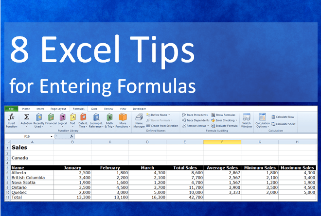
If you're looking to discover overall sales profits from a number of marketed systems, for instance, the selection formula in Excel is ideal for you. Below's exactly how you 'd do it: To start utilizing the range formula, type "=SUM," as well as in parentheses, enter the very first of 2 (or 3, or four) varieties of cells you 'd such as to multiply together.

This means reproduction. Following this asterisk, enter your 2nd series of cells. You'll be increasing this 2nd variety of cells by the first. Your progress in this formula should currently appear like this: =AMOUNT(C 2: C 5 * D 2:D 5) Ready to press Go into? Not so quickly ... Since this formula is so complex, Excel books a different key-board command for selections.

This will identify your formula as a variety, wrapping your formula in brace personalities as well as successfully returning your item of both varieties incorporated. In income estimations, this can minimize your time and also effort significantly. See the final formula in the screenshot over. The COUNT formula in Excel is denoted =MATTER(Begin Cell: End Cell).

For instance, if there are 8 cells with gone into worths between A 1 and also A 10, =MATTER(A 1: A 10) will certainly return a value of 8. The MATTER formula in Excel is particularly valuable for huge spread sheets, where you wish to see the number of cells contain real entrances. Do not be misleaded: This formula will not do any type of math on the values of the cells themselves.

Excel If Formula - Truths

Using the formula in vibrant above, you can easily run a matter of current cells in your spread sheet. The outcome will look a something like this: To carry out the typical formula in Excel, get in the values, cells, or variety of cells of which you're determining the average in the layout, =AVERAGE(number 1, number 2, and so on) or =STANDARD(Beginning Worth: End Worth).

Finding the average of a range of cells in Excel maintains you from needing to locate individual sums and afterwards doing a separate division formula on your total. Using =STANDARD as your preliminary text entry, you can let Excel do all the benefit you. For reference, the standard of a group of numbers amounts to the sum of those numbers, split by the variety of items in that group.

This will certainly return the sum of the values within a preferred range of cells that all meet one requirement. For instance, =SUMIF(C 3: C 12,"> 70,000") would certainly return the amount of values in between cells C 3 and also C 12 from only the cells that are above 70,000. Allow's claim you intend to establish the earnings you generated from a list of leads who are related to particular area codes, or calculate the amount of specific staff members' wages-- yet only if they drop above a particular quantity.

With the SUMIF function, it doesn't have to be-- you can conveniently accumulate the amount of cells that meet certain standards, like in the income example over. The formula: =SUMIF(variety, criteria, [sum_range] Range: The array that is being examined using your requirements. Criteria: The criteria that determine which cells in Criteria_range 1 will certainly be totaled [Sum_range]: An optional array of cells you're mosting likely to add up along with the first Range entered.

In the instance listed below, we wished to compute the amount of the wages that were more than $70,000. The SUMIF feature built up the dollar amounts that went beyond that number in the cells C 3 through C 12, with the formula =SUMIF(C 3: C 12,"> 70,000"). The TRIM formula in Excel is represented =TRIM(message).

The 30-Second Trick For Vlookup Excel

As an example, if A 2 includes the name" Steve Peterson" with undesirable spaces prior to the initial name, =TRIM(A 2) would return "Steve Peterson" without any areas in a new cell. Email and file sharing are terrific devices in today's work environment. That is, up until among your coworkers sends you a worksheet with some actually fashionable spacing.

As opposed to painstakingly removing as well as adding spaces as required, you can cleanse up any kind of uneven spacing making use of the TRIM function, which is made use of to remove added rooms from information (other than for solitary areas in between words). The formula: =TRIM(text). Text: The text or cell from which you intend to eliminate rooms.

To do so, we got in =TRIM("A 2") right into the Formula Bar, and also reproduced this for each and every name listed below it in a new column alongside the column with undesirable rooms. Below are a few other Excel formulas you may find helpful as your information monitoring needs grow. Allow's claim you have a line of message within a cell that you wish to damage down into a couple of different segments.

Function: Made use of to extract the very first X numbers or personalities in a cell. The formula: =LEFT(message, number_of_characters) Text: The string that you want to extract from. Number_of_characters: The number of characters that you desire to remove beginning with the left-most personality. In the instance listed below, we got in =LEFT(A 2,4) right into cell B 2, and also copied it into B 3: B 6.

Objective: Used to draw out characters or numbers in the center based on position. The formula: =MID(text, start_position, number_of_characters) Text: The string that you wish to remove from. Start_position: The placement in the string that you desire to start drawing out from. For example, the first position in the string is 1.

The Ultimate Guide To Countif Excel

In this example, we entered =MID(A 2,5,2) into cell B 2, as well as replicated it right into B 3: B 6. That allowed us to extract both numbers beginning in the fifth position of the code. Function: Used to extract the last X numbers or personalities in a cell. The formula: =RIGHT(message, number_of_characters) Text: The string that you desire to remove from.

excel formulas upper and lowercase excel formulas most used excel formulas mula